User Manual

ethograph is a GUI for visualizing and segmenting multimodal behavioural recordings.

Install

uv tool install --python 3.12 "ethograph[gui,audio]"

Launch with ethograph launch, or the desktop shortcut. See Installation for detailed instructions and troubleshooting.

Multimodal visualization

Ethograph allows you to visualize a number of different data modalities:

Data	Shown as	File formats / loaders
Video	multi-panel video	.mp4, .avi, .mov, .mkv (via pyav and pynaviz)
Pose / BoundingBox	Overlay on video	.h5, .csv, .slp (DLC, SLEAP, LightningPose, … via movement)
Audio	Waveform + spectrogram	.wav, .flac, .ogg, .mp3 (via audioio)
Electrophysiology	Multi-channel trace	.dat, .bin, .raw via phylib, and many more formats via Neo
Spike-sorted units	Raster / PSTH	Kilosort folder, .nwb file, pynapple.TsGroup
Features	Line plots / heatmaps	Kinematics, firing rates, latent variables, model outputs, etc.

Feature data can be loaded via three backends:

Backend	Object	File format
xarray	xarray.Dataset / TrialTree	.nc
Pynapple	Tsd / TsdFrame	.npz or folder
NWB	.nwb (loaded via pynapple)	.nwb
numpy	plain array	.npy

Unlike a plain numpy array, the top three formats carry explicit timestamps with each value. This allows ethograph to automatically align data of different sampling rates and modalities (video, audio & electrophysiology).

Note

.npy only supports (T, D) dimensional data. It can be loaded via drag & drop, you’ll be asked for the sampling rate of each timestamp (T), and it is converted internally into a timestamped object.

Loading your data

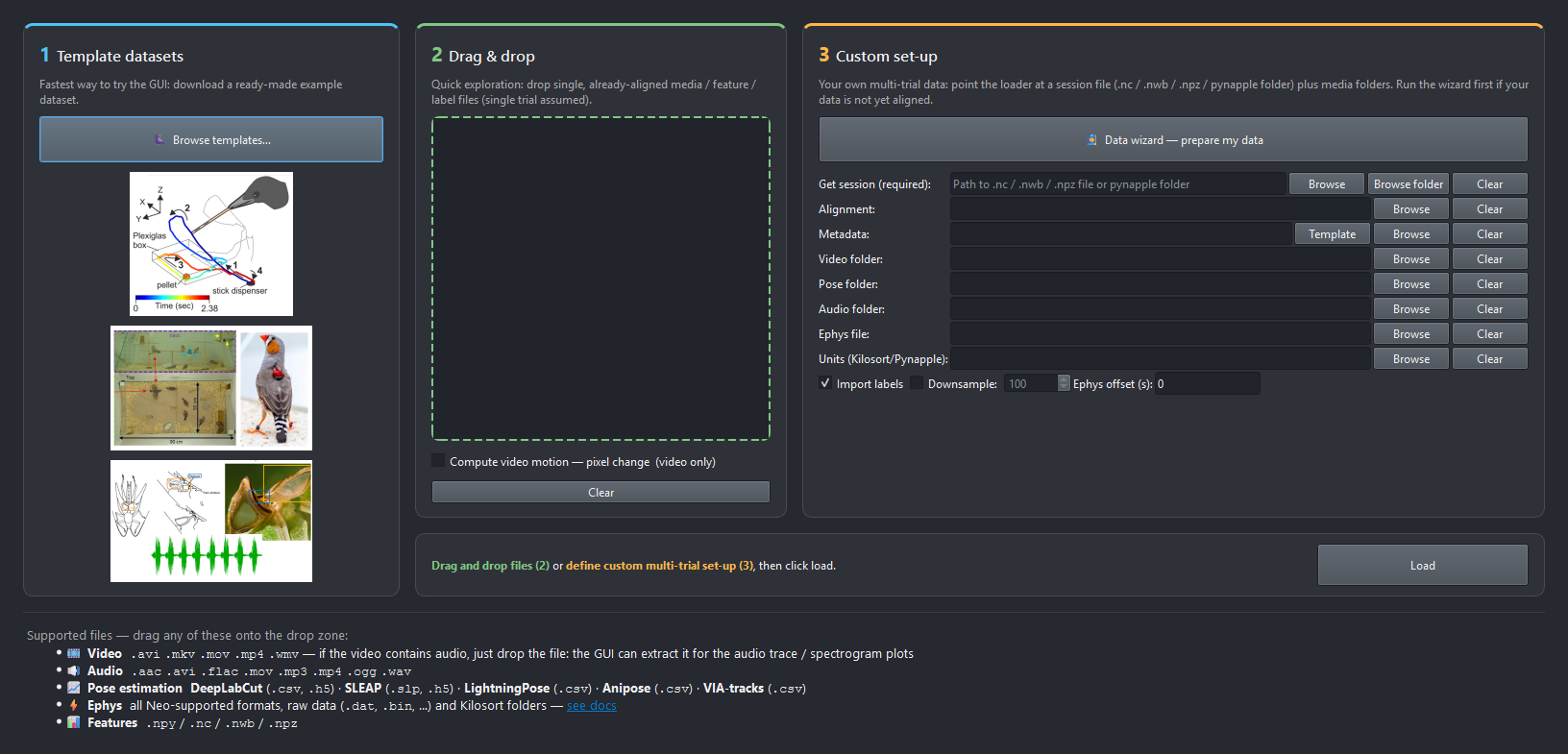
Launching opens the start page. It lists the supported file types along the bottom and offers three ways in:

Which entry point?

New here? Start with Template datasets (1) — example data of cool animal behaviours (🐦‍⬛🐦🎶🦗🐀) that loads in one click. See more here: examples gallery.

For your own data, the question is not how many files you have — drag & drop takes many — but how they are arranged across devices and trials.

Your data	Use
One trial, many devices. Files that start together and cover the same stretch of time — four cameras, three microphones, pose per camera.	Drag & drop (2), Several cameras/mics filming one trial
Many trials, one device. One file per trial per stream — trial001.mp4, trial002.mp4, …, optionally with matching pose and audio files.	Drag & drop (2), Several trials of one device
Many trials and many devices — e.g. 20 trials filmed by 2 cameras with 1 microphone (40 videos + 20 audio files); streams needing offsets — ephys on its own clock, trial windows carved out of a continuous recording; or an existing session file (.nc with trials, .nwb, pynapple).	Custom set-up (3)

Drag & drop

Pick a layout in the drop card’s dropdown, drop the files, click Load. Frame rates, sample rates and durations are read from the files themselves. You are only asked for what cannot be inferred: the source software of an ambiguous .h5/.csv pose file, the sampling rate of a .npy, or the camera order when several videos and pose files arrive together.

Several cameras/mics filming one trial (default): several videos become cam-1, cam-2, … (each its own view, one shared playhead); several audio files become mic-1, mic-2, … A multichannel .wav is split into channels automatically.

Several trials of one device: the files of each stream are natural-sorted and paired one per trial, so trial001.mp4 goes with trial001.h5. Every stream must hold the same number of files; the result is a multi-trial session you navigate trial by trial.

In both layouts, pose files also gain velocity, acceleration and speed per keypoint on load.

Project folder — keep your drops

A drop is a quick look by default: the alignment it builds lives in a temp folder and is gone next time. Choose a Project folder in the bar above the cards to keep them instead. Every drop made while it is set lands in the project’s sessions/ folder, one timestamped folder per drop (2026-09-06_21-47-12/), holding the alignment file, anything derived from the drop and the panel layout you left it with. The drop card then lists them under Reopen a previous drop…: pick one, click Load, and the session comes back as it was. Your media and data files stay where they are — nothing is copied into the project.

Custom set-up

Point the loader at a session file (.nc, .nwb, .npz or a pynapple folder) plus, optionally, the folders holding your media. Ephys recorded on its own clock gets an Ephys offset (s) field here.

The I/O section offers a lot of flexibility, but may be overly complex for your data. In many cases the Data wizard button can guide you through organizing and temporally aligning your media streams — including many trials across several cameras and microphones — into a session.nc. For more complex scenarios you may have to write a custom Python script:

See Bring your own data for the full workflow and dataset schema, and Ephys recordings for ephys formats and Kilosort.

Labelling

Ethograph is a labelling GUI for marking the onset and offset of behavioural events. Press a number key to select a label class, click on the timeseries plot to mark the onset, click again to mark the offset, then press V to play back the segment you just labelled.

The labels documentation includes more info on how to:

• label in the GUI

• define new label categories (mapping.txt)

• deal with labels overlapping in time (label branches)

• import labels from other formats (Pynapple, NWB, BORIS, audacity, Raven, …)

• export labels

Trial metadata

Per-trial conditions (stimulus, reward, pellet count, …) live in a small table — a {stem}_metadata.tsv next to your data, or the NWB trials table — and show up as the trials table at the top of the Navigation section, where each column becomes a filter. See Trial metadata.

Important

The trials table is the one place trials are included or excluded — and it applies to everything. Filter num_pellets to 1, 2 (not 0) and every operation sees only those trials: navigation, label/sequence jumps, changepoint correction, curation (Ctrl+C, inspect mode, frame-by-frame review, the label and video grids), model training and model inference. A label in a filtered-out trial is not visited, curated, trained on or predicted over until you widen the filter. No dialog has a trial filter of its own; each one tells you how many trials it will run over.

Two more things worth knowing: EthoGraph keeps a curated column in that table itself (yes once every label of a trial is manual or curated, otherwise no — see Curating labels), and metadata edits save on their own, about a second after you stop typing — Ctrl+S is only for labels.

The interface

The layout is responsive and panel-based: every plot, video and trace lives in its own panel that you can drag, stack, tab, float and resize freely.

• Click a panel to edit it. The right sidebar is context-sensitive — clicking a panel shows the settings for that panel (e.g. the feature and its dimensions for a line plot, or the channel for an audio panel).

• Add panels with the ➕ Add panel button (bottom-left of the window, or Shift+N): drag a data source onto the plot area, or press Enter to drop it in the default spot. Remove any panel with its ✕. You can open as many as you like — e.g. the same feature as both a line plot and a heatmap.

Which individual a panel shows

With more than one individual in the dataset, every panel is in one of two modes, shown in its title:

speed — bird_1 (sidebar)    follows the Individual combo
speed — bird_2 (pinned)     ignores it

• The Individual combo sets what every (sidebar) panel shows, and the default for new panels.

• 📌 next to the combo pins the last clicked panel (line plot, heatmap or camera view) to one individual, or sets it back to Follow sidebar.

• A pinned line plot/heatmap selects that individual from its feature; a pinned camera view shows only that individual’s pose overlay; a panel pinned to individual X only shows labels where X is the actor.

To compare two birds side by side: add two duplicate lineplots via ➕ Add panel. Then for one of them, click 📌 → bird_2. Switching the combo now moves only the original.

Video & audio playback

Two things are easy to miss when you first play back a recording:

• The red timeline marker tracks exact time, not the video frame. Video is discrete frames, but audio and other signals have far finer resolution, so clicking a plot places the marker (and any label) at the exact time you clicked — the video just seeks to the nearest frame as a visual reference.

• Only “Audio-synced” playback plays sound. The playback mode dropdown in the bottom bar also offers silent “Smooth” and “Real-time” modes; pick Audio-synced whenever you need to hear the audio locked to the video.

See Video & Audio playback for the full details, including playback speed/pitch, video proxies for smooth scrubbing, and which audio channel Play uses.

Feature dropdowns

To showcase some ethograph functionalities, we will use pose data from a carrion crow performing a tool-use task [Moll et al., 2025]. The xarray.Dataset is from one behavioural trial, and shows position, velocity, speed, and acceleration for 3 keypoints tracked in 3D.

import ethograph as eto

ds = eto.sample_data()
ds[["position", "velocity", "speed"]]

<xarray.Dataset> Size: 190kB
Dimensions:     (time: 1077, space: 3, keypoint: 3, individual: 1)
Coordinates:
  * time        (time) float64 9kB 0.0 0.005 0.01 0.015 ... 5.37 5.375 5.38
  * space       (space) <U1 12B 'x' 'y' 'z'
  * keypoint    (keypoint) <U8 96B 'beakTip' 'stickTip' 'pellet'
  * individual  (individual) <U5 20B 'Crow1'
Data variables:
    position    (time, space, keypoint, individual) float64 78kB ...
    velocity    (time, space, keypoint, individual) float64 78kB ...
    speed       (time, keypoint, individual) float64 26kB ...
Attributes:
    source_software:  DeepLabCut
    ds_type:          poses
    fps:              200.0
    time_unit:        seconds
    source_file:      c:/Users/aksel/Documents/Code/ethograph/data/Moll2025/2...
    trial:            41
    pellet_position:  right

xarray.Dataset

• Dimensions:
  • time: 1077
  • space: 3
  • keypoint: 3
  • individual: 1
• Coordinates: (4)
  • time
    (time)
    float64
    0.0 0.005 0.01 ... 5.37 5.375 5.38

    array([0.000e+00, 5.000e-03, 1.000e-02, ..., 5.370e+00, 5.375e+00, 5.380e+00],
          shape=(1077,))

  • space
    (space)
    <U1
    'x' 'y' 'z'

    array(['x', 'y', 'z'], dtype='<U1')

  • keypoint
    (keypoint)
    <U8
    'beakTip' 'stickTip' 'pellet'

    array(['beakTip', 'stickTip', 'pellet'], dtype='<U8')

  • individual
    (individual)
    <U5
    'Crow1'

    array(['Crow1'], dtype='<U5')

• Data variables: (3)
  • position
    (time, space, keypoint, individual)
    float64
    ...

    [9693 values with dtype=float64]

  • velocity
    (time, space, keypoint, individual)
    float64
    ...

    [9693 values with dtype=float64]

  • speed
    (time, keypoint, individual)
    float64
    ...

    [3231 values with dtype=float64]

• Attributes: (7)

  source_software :

  DeepLabCut

  ds_type :

  poses

  fps :

  200.0

  time_unit :

  seconds

  source_file :

  c:/Users/aksel/Documents/Code/ethograph/data/Moll2025/2024-12-18_041_Crow1_DLC_3D.csv

  trial :

  41

  pellet_position :

  right

Notice the dimensions:

Feature	Dimensions
position	(time, space, keypoint, individual)
velocity	(time, space, keypoint, individual)
speed	(time, keypoint, individual)

With xarray.DataArray, you can use sel() to pick a specific keypoint, spatial axis, and individual:

# Standard xarray .sel — works when all dimensions exist
print(f"Dims: {ds['position'].dims}, Shape: {ds['position'].shape}")
beak_x = ds["position"].sel(keypoint="beakTip", space="x", individual="Crow1")
print(f"Dims: {beak_x.dims}, Shape: {beak_x.shape}")

Dims: ('time', 'space', 'keypoint', 'individual'), Shape: (1077, 3, 3, 1)
Dims: ('time',), Shape: (1077,)

---

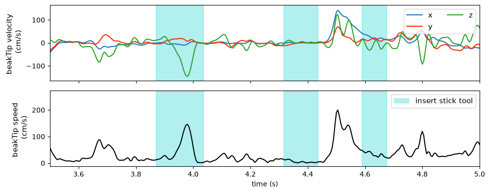
In the GUI, you can switch between features using the Feature dropdown and select (sel()) a unique combination of feature dimensions. In the video below, the user switches from the feature speed to velocity, with the selection dimensions individual=crow1, keypoint=beakTip and space=["x", "y", "z"] (All checkbox ticked). Thanks to sel_valid(), any invalid dimensions are ignored (e.g. it’s not problematic that speed does not have a space dimension).

At the end of the video and in the plot below, one can see that particularly velocity for keypoint=beakTip and space=z (green line) defines segmentation boundaries of the crows downward movement, inserting the stick tool into the dispenser.

Show code cell source

Hide code cell source

import matplotlib.patches as mpatches
import matplotlib.pyplot as plt
import numpy as np

from ethograph.labels.intervals import add_interval, empty_intervals
from ethograph.labels.plots import plot_label_segments

sel = {"keypoint": "beakTip", "individual": "Crow1"}

# 3 labelled intervals (real onsets from the Moll2025 dataset)
label_color = np.array([0, 204, 204]) / 255.0  # _LABEL_COLORS[10]
labels_df = empty_intervals()
labels_df = add_interval(labels_df, 3.87, 4.035, 10, "Crow1")
labels_df = add_interval(labels_df, 4.315, 4.435, 10, "Crow1")
labels_df = add_interval(labels_df, 4.588757756, 4.674700055, 10, "Crow1")

label_mappings = {10: {"name": "stickInDisp", "color": label_color, "order": 10, "branch": 0}}

fig, axes = plt.subplots(2, 1, figsize=(10, 4), sharex=True)

# velocity x, y, z
for i, (axis_name, color) in enumerate(zip(["x", "y", "z"], ["#1f77b4", "#ff2a0e", "#2ca02c"])):
    vel, _ = eto.sel_valid(ds["velocity"].sel(space=axis_name), sel)
    axes[0].plot(ds.time, vel, color=color, label=axis_name)
axes[0].set_ylabel("beakTip velocity \n (cm/s)", fontsize=11)
axes[0].legend(loc="upper right", fontsize=11, ncol=2)
plot_label_segments(axes[0], labels_df, label_mappings, individual="Crow1", is_main=True, alpha=0.3)

# speed
spd, _ = eto.sel_valid(ds["speed"], sel)
axes[1].plot(ds.time, spd, color="#000305")
axes[1].set_ylabel("beakTip speed \n (cm/s)", fontsize=11)
plot_label_segments(axes[1], labels_df, label_mappings, individual="Crow1", is_main=True, alpha=0.3)

axes[1].set_xlabel("time (s)")
insert_stick_patch = mpatches.Patch(
    facecolor=label_color,
    alpha=0.3,
    edgecolor="none",
    label="insert stick tool",
)

handles, labels = axes[0].get_legend_handles_labels()
axes[1].legend(
    [insert_stick_patch],
    ["insert stick tool"],
    loc="upper right",
    fontsize=11,
    ncol=4,
)

for ax in axes:
    ax.set_xlim(3.5, 5.0)


plt.tight_layout()
plt.show()

Changepoints

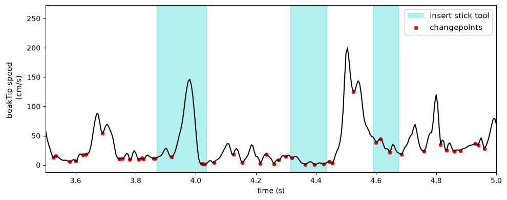
Besides looking at the z-velocity, one can also identify good candidates for segmentation boundaries by looking at where there are minima or turning points in the beakTip speed curve. We call these kinematic changepoints.

Show code cell source

Hide code cell source

import matplotlib.patches as mpatches
import matplotlib.pyplot as plt
import numpy as np

from ethograph.labels.intervals import add_interval, empty_intervals
from ethograph.labels.plots import plot_label_segments

sel = {"keypoint": "beakTip", "individual": "Crow1"}

# 3 labelled intervals (real onsets from the Moll2025 dataset)
label_color = np.array([0, 204, 204]) / 255.0  # _LABEL_COLORS[10]
labels_df = empty_intervals()
labels_df = add_interval(labels_df, 3.87, 4.035, 10, "Crow1")
labels_df = add_interval(labels_df, 4.315, 4.435, 10, "Crow1")
labels_df = add_interval(labels_df, 4.588757756, 4.674700055, 10, "Crow1")

label_mappings = {10: {"name": "stickInDisp", "color": label_color, "order": 10, "branch": 0}}

fig = plt.subplots(1, 1, figsize=(10, 4), sharex=True)

# speed
spd, _ = eto.sel_valid(ds["speed"], sel)
plt.plot(ds.time, spd, color="#000305")

troughs = ds["speed_troughs"].sel(keypoint="beakTip", individual="Crow1").values
trough_idx = np.where(troughs == 1)[0]
turning_points = ds["speed_turning_points"].sel(keypoint="beakTip", individual="Crow1").values
turning_points_idx = np.where(turning_points == 1)[0]
changepoints_idx = np.sort(np.concatenate([trough_idx, turning_points_idx]))
plt.scatter(ds.time[changepoints_idx], spd[changepoints_idx], s=20, c="r", label="changepoints")
plt.ylabel("beakTip speed \n (cm/s)", fontsize=11)
plot_label_segments(plt, labels_df, label_mappings, individual="Crow1", is_main=True, alpha=0.3)

plt.xlabel("time (s)")
insert_stick_patch = mpatches.Patch(
    facecolor=label_color,
    alpha=0.3,
    edgecolor="none",
    label="insert stick tool",
)

handles, labels = plt.gca().get_legend_handles_labels()
plt.legend(
    [insert_stick_patch, *handles],
    ["insert stick tool", *labels],
    loc="upper right",
    fontsize=11,
)

plt.xlim(3.5, 5.0)
plt.tight_layout()
plt.show()

Storing trials: Dataset vs TrialTree

Back at the start we split loading into one recording versus trials. That choice decides how you load; this section shows what it looks like on disk for the xarray backend. A session.nc can hold either shape, and the GUI accepts both.

Plain Dataset — a single xr.Dataset saved with xarray.Dataset.to_netcdf(). Loaded as one trial:

import xarray as xr

ds = xr.Dataset(...)
ds.to_netcdf("session.nc")
# -> GUI loads this as one trial

TrialTree — wraps one xr.Dataset per trial into a single .nc, and is how multi-trial data is stored on the xarray side (pynapple uses an IntervalSet; NWB uses its nwb.trials table):

import ethograph as eto

# Multiple trials: one Dataset per trial
dt = eto.from_datasets([ds_trial1, ds_trial2, ds_trial3])
dt.save("session.nc")

# Access individual trials
ds = dt.trial(1)      # by ID
ds = dt.itrial(0)     # by index

One session-long xr.Dataset plus trial start/stop times? Pass both to from_continuous(). The times can be a pd.DataFrame with trial, start_time and stop_time columns (in seconds, on the dataset’s time axis) or a pynapple.IntervalSet. Each trial becomes its own window, with time starting at 0:

trials = pd.DataFrame({"trial": [1, 2], "start_time": [0.0, 120.0], "stop_time": [100.0, 250.0]})
dt = eto.from_continuous(ds, trials)
dt.save("session.nc")

Storing trials is only half the job: the GUI also needs to know which video, audio and pose files belong to each trial, which lives in a separate alignment file. Bring your own data covers both ends — the dataset schema and the alignment — and TrialTree documents the full TrialTree API.

Template datasets

Ready-made datasets with video, features and labels already in place, downloaded from the start page. The notebooks that built them are in the examples gallery.

Tool-using crows [Moll et al., 2025] — Learned precision tool use in carrion crows. Two trials with video, 3D pose (DeepLabCut), kinematics, and video features.

Lockbox [Reiske et al., 2026] — Behaviour recognition for mice solving mechanical puzzle lockboxes. Six trials with multi-camera video and pose.

Zebra finches in BirdPark [Rüttimann et al., 2025] — Multimodal dataset of zebra finch groups with synchronized video, microphone arrays, and backpack-mounted accelerometers.

Cricket stridulation — Sound production in Pholidoptera littoralis with synchronized video, audio, and DeepLabCut pose.