User Manual

ethograph visualizes behavioural recordings across modalities:

Data	Shown as	File formats / loaders
Video	pygfx viewer (via pynaviz)	.mp4 (recommended), .avi, .mov (via pyav)
Pose/ BoundingBox	Overlay on video	.h5, .csv (DLC, SLEAP, LightningPose, … via movement)
Audio	Waveform + spectrogram	.wav, .mp3 (via audioio)
Electrophysiology	Multi-channel trace	.dat, .bin, .raw via phylib and supported extensions via Neo
Spike-sorted units	Raster / PSTH	Kilosort folder, .nwb file, pynapple.TsGroup
Features	Line plots / heatmaps	Kinematics, firing rates, latent variables, model outputs, etc.

---

Feature data can be loaded via three backends:

Backend	Object	File format
xarray	xarray.Dataset / TrialTree	.nc
Pynapple	Tsd / TsdFrame	.npz or folder
NWB	.nwb (loaded via pynapple)	.nwb

Unlike a plain numpy array, all three formats carry explicit timestamps with each value. This allows ethograph to automatically align data of different sampling rates and modalities (video, audio & electrophysiology).

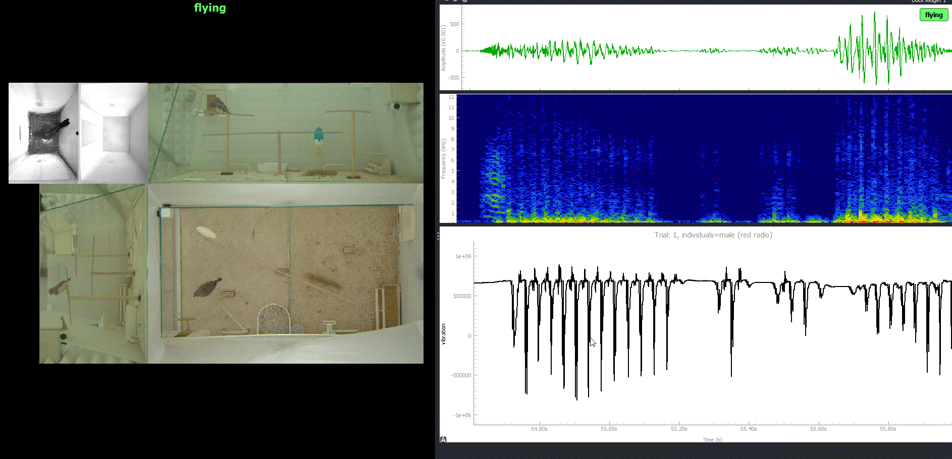
Labelling

Ethograph is a labelling GUI for marking the onset and offset of behavioural events. Press a number key to select a label class, click on the timeseries plot to mark the onset, click again to mark the offset, then press V to play back the segment you just labelled.

The labels documentation includes more info on how to:

• label in the GUI

• define new label categories (mapping.txt)

• deal with labels overlapping in time (label branches)

• import labels from other formats (Pynapple, NWB, BORIS, audacity, Raven, …)

• export labels

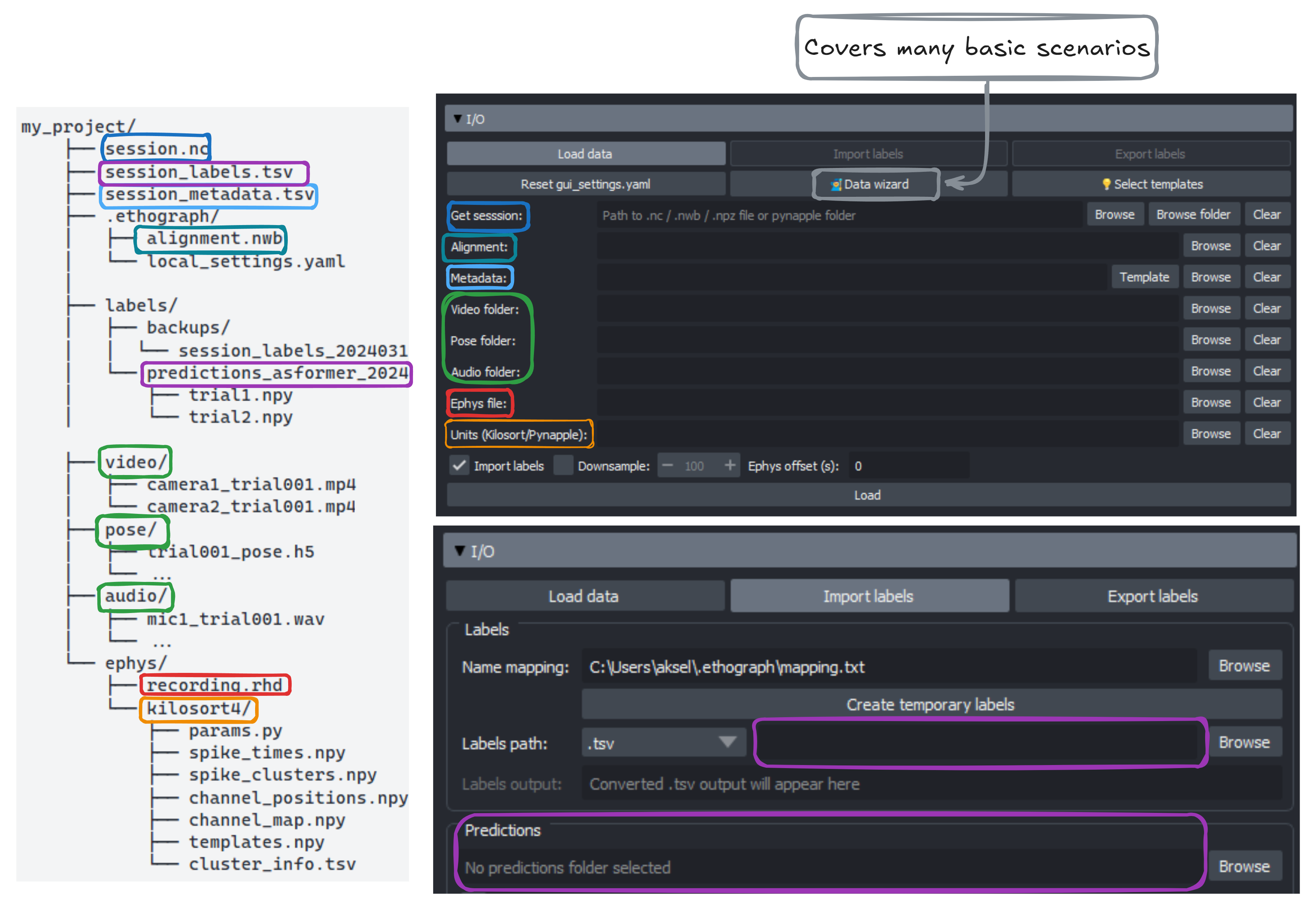
Importing data

The I/O section (see image below) offers a lot of flexibility, but may be overly complex for your data. As a first starting point, have a look at the Getting Started Wizard. In many cases, the Data wizard can guide you through the steps to organize & temporally align your different data/media streams. For more complex scenarios, you may have to write a custom Python script.

Feature dropdowns

To showcase some ethograph functionalities, we will use pose data from a carrion crow performing a tool-use task (Moll et al., 2025¹). The xarray.Dataset is from one behavioural trial, and shows position, velocity, speed, and acceleration for 3 keypoints tracked in 3D.

import ethograph as eto

ds = eto.sample_data()
ds[["position", "velocity", "speed"]]

<xarray.Dataset> Size: 206kB
Dimensions:      (time: 1169, space: 3, keypoints: 3, individuals: 1)
Coordinates:
  * time         (time) float64 9kB 0.0 0.005 0.01 0.015 ... 5.83 5.835 5.84
  * space        (space) <U1 12B 'x' 'y' 'z'
  * keypoints    (keypoints) <U8 96B 'beakTip' 'stickTip' 'pellet'
  * individuals  (individuals) <U5 20B 'Crow1'
Data variables:
    position     (time, space, keypoints, individuals) float64 84kB ...
    velocity     (time, space, keypoints, individuals) float64 84kB ...
    speed        (time, keypoints, individuals) float64 28kB ...
Attributes:
    source_software:  DeepLabCut
    ds_type:          poses
    fps:              200.0
    time_unit:        seconds
    source_file:      C:/Users/aksel/Documents/Code/EthoGraph/data/Moll2025/2...
    trial:            115
    bird:             Crow1
    session_date:     2024-12-17
    pellet_position:  left
    human_verified:   1

xarray.Dataset

• Dimensions:
  • time: 1169
  • space: 3
  • keypoints: 3
  • individuals: 1
• Coordinates: (4)
  • time
    (time)
    float64
    0.0 0.005 0.01 ... 5.83 5.835 5.84

    array([0.000e+00, 5.000e-03, 1.000e-02, ..., 5.830e+00, 5.835e+00, 5.840e+00],
          shape=(1169,))

  • space
    (space)
    <U1
    'x' 'y' 'z'

    array(['x', 'y', 'z'], dtype='<U1')

  • keypoints
    (keypoints)
    <U8
    'beakTip' 'stickTip' 'pellet'

    array(['beakTip', 'stickTip', 'pellet'], dtype='<U8')

  • individuals
    (individuals)
    <U5
    'Crow1'

    array(['Crow1'], dtype='<U5')

• Data variables: (3)
  • position
    (time, space, keypoints, individuals)
    float64
    ...

    type :

    features

    [10521 values with dtype=float64]

  • velocity
    (time, space, keypoints, individuals)
    float64
    ...

    type :

    features

    [10521 values with dtype=float64]

  • speed
    (time, keypoints, individuals)
    float64
    ...

    type :

    features

    [3507 values with dtype=float64]

• Attributes: (10)

  source_software :

  DeepLabCut

  ds_type :

  poses

  fps :

  200.0

  time_unit :

  seconds

  source_file :

  C:/Users/aksel/Documents/Code/EthoGraph/data/Moll2025/2024-12-17_115_Crow1_DLC_3D.csv

  trial :

  115

  bird :

  Crow1

  session_date :

  2024-12-17

  pellet_position :

  left

  human_verified :

  1

Notice the dimensions:

Feature	Dimensions
position	(time, space, keypoint, individual)
velocity	(time, space, keypoint, individual)
speed	(time, keypoint, individual)

With xarray.DataArray, you can use sel() to pick a specific keypoint, spatial axis, and individual:

# Standard xarray .sel — works when all dimensions exist
beak_x = ds["position"].sel(keypoint="beakTip", space="x", individual="Crow1")
print(f"position with .sel: shape {beak_x.shape}")

# But speed has no 'space' dimension — .sel raises an error:
try:
    ds["speed"].sel(keypoint="beakTip", space="x", individual="Crow1")
except (KeyError, ValueError) as e:
    print(f"speed with .sel:   {type(e).__name__}: {e}")

---

In the GUI, you can switch between features using the Feature dropdown and select (sel()) a unique combination of feature dimensions. In the video below, the user switches from the feature speed to velocity, with the selection dimensions individual=crow1, keypoint=beakTip and space=["x", "y", "z"] (All checkbox ticked). Thanks to sel_valid(), any invalid dimensions are ignored (e.g. it’s not problematic that speed does not have a space dimension).

At the end of the video and in the plot below, one can see that particularly velocity for keypoint=beakTip and space=z (green line) defines segmentation boundaries of the crows downward movement, inserting the stick tool into the dispenser.

Show code cell source

Hide code cell source

import matplotlib.patches as mpatches
import matplotlib.pyplot as plt
import numpy as np

from ethograph.labels.intervals import add_interval, empty_intervals
from ethograph.labels.plots import plot_label_segments

sel = {"keypoint": "beakTip", "individual": "Crow1"}

# 3 labelled intervals (real onsets from the Moll2025 dataset)
label_color = np.array([0, 204, 204]) / 255.0  # _LABEL_COLORS[10]
labels_df = empty_intervals()
labels_df = add_interval(labels_df, 3.87, 4.035, 10, "Crow1")
labels_df = add_interval(labels_df, 4.315, 4.435, 10, "Crow1")
labels_df = add_interval(labels_df, 4.588757756, 4.674700055, 10, "Crow1")

label_mappings = {10: {"name": "stickInDisp", "color": label_color, "order": 10, "branch": 0}}

fig, axes = plt.subplots(2, 1, figsize=(10, 4), sharex=True)

# velocity x, y, z
for i, (axis_name, color) in enumerate(zip(["x", "y", "z"], ["#1f77b4", "#ff2a0e", "#2ca02c"])):
    vel, _ = eto.sel_valid(ds["velocity"].sel(space=axis_name), sel)
    axes[0].plot(ds.time, vel, color=color, label=axis_name)
axes[0].set_ylabel("beakTip velocity \n (cm/s)", fontsize=11)
axes[0].legend(loc="upper right", fontsize=11, ncol=2)
plot_label_segments(axes[0], labels_df, label_mappings, individual="Crow1", is_main=True, alpha=0.3)

# speed
spd, _ = eto.sel_valid(ds["speed"], sel)
axes[1].plot(ds.time, spd, color="#000305")
axes[1].set_ylabel("beakTip speed \n (cm/s)", fontsize=11)
plot_label_segments(axes[1], labels_df, label_mappings, individual="Crow1", is_main=True, alpha=0.3)

axes[1].set_xlabel("time (s)")
insert_stick_patch = mpatches.Patch(
    facecolor=label_color,
    alpha=0.3,
    edgecolor="none",
    label="insert stick tool",
)

handles, labels = axes[0].get_legend_handles_labels()
axes[1].legend(
    [insert_stick_patch],
    ["insert stick tool"],
    loc="upper right",
    fontsize=11,
    ncol=4,
)

for ax in axes:
    ax.set_xlim(3.5, 5.0)


plt.tight_layout()
plt.show()

Changepoints

Besides looking at the z-velocity, one can also identify good candidates for segmentation boundaries by looking at where there are minima or turning points in the beakTip speed curve. We call these kinematic changepoints.

Show code cell source

Hide code cell source

import matplotlib.patches as mpatches
import matplotlib.pyplot as plt
import numpy as np

from ethograph.labels.intervals import add_interval, empty_intervals
from ethograph.labels.plots import plot_label_segments

sel = {"keypoint": "beakTip", "individual": "Crow1"}

# 3 labelled intervals (real onsets from the Moll2025 dataset)
label_color = np.array([0, 204, 204]) / 255.0  # _LABEL_COLORS[10]
labels_df = empty_intervals()
labels_df = add_interval(labels_df, 3.87, 4.035, 10, "Crow1")
labels_df = add_interval(labels_df, 4.315, 4.435, 10, "Crow1")
labels_df = add_interval(labels_df, 4.588757756, 4.674700055, 10, "Crow1")

label_mappings = {10: {"name": "stickInDisp", "color": label_color, "order": 10, "branch": 0}}

fig = plt.subplots(1, 1, figsize=(10, 4), sharex=True)

# speed
spd, _ = eto.sel_valid(ds["speed"], sel)
plt.plot(ds.time, spd, color="#000305")

troughs = ds["speed_troughs"].sel(keypoint="beakTip", individual="Crow1").values
trough_idx = np.where(troughs == 1)[0]
turning_points = ds["speed_turning_points"].sel(keypoint="beakTip", individual="Crow1").values
turning_points_idx = np.where(turning_points == 1)[0]
changepoints_idx = np.sort(np.concatenate([trough_idx, turning_points_idx]))
plt.scatter(ds.time[changepoints_idx], spd[changepoints_idx], s=20, c="r", label="changepoints")
plt.ylabel("beakTip speed \n (cm/s)", fontsize=11)
plot_label_segments(plt, labels_df, label_mappings, individual="Crow1", is_main=True, alpha=0.3)

plt.xlabel("time (s)")
insert_stick_patch = mpatches.Patch(
    facecolor=label_color,
    alpha=0.3,
    edgecolor="none",
    label="insert stick tool",
)

handles, labels = plt.gca().get_legend_handles_labels()
plt.legend(
    [insert_stick_patch, *handles],
    ["insert stick tool", *labels],
    loc="upper right",
    fontsize=11,
)

plt.xlim(3.5, 5.0)
plt.tight_layout()
plt.show()

Data requirements summary

	xarray	Pynapple	NWB
File format	.nc via TrialTree	.npz or folder	.nwb
Required attrs	trial, fps	(none)	(NWB standard)
Features	Any data_var with a time dim	Any Tsd / TsdFrame	TimeSeries in processing
Individuals	coords["individual"]	Separate objects	One subject per file
Trials	One Dataset per trial	IntervalSet	nwb.trials table

See Data Format Requirements for full specifications across all three backends.

Operations across backends

Operation	xarray / TrialTree	Pynapple	NWB
Load	open()	load_nap_data()	load_nap_data()
Restrict	sel()	restrict()	Via pynapple
Select dims	sel_valid()	Column indexing on TsdFrame	Via pynapple
Build	from_datasets()	save_file()	NWBHDF5IO
Alignment	.ethograph/alignment.nwb	.ethograph/alignment.nwb	In source .nwb
Iterate trials	trial_items()	restrict()	Via pynapple

References

Moll, F. W., Würzler, J., & Nieder, A. (2025). Learned precision tool use in carrion crows. Current Biology, 35(19), 4845-4852.e3. https://doi.org/10.1016/j.cub.2025.08.033